Contact	Research	Publications	Teaching	Software	Links
Dr. Philip Siegmann

Research

• Applied Optics
• New Optical Methods
  
• In-line surface defects detection and cuantification on ultrafine wires. Analysing the geometrical part of a conical diffracted laser beam generated after impinging with it on a wire, we are able to detect surface defects (usualy longitudinal structures) on wires with diameter between 30 to 600 micrometers. We developed an optical system (shown in Fig.1) and the necessary image processing algorithms based on this method that allows real time surface inspection and evaluation of the whole 360 degree of the wire surface contour. See references [10] and [15] in Publications for more details. This was a result of an EU project SMT4-CT97-2184 (DEFCYL).

  (a)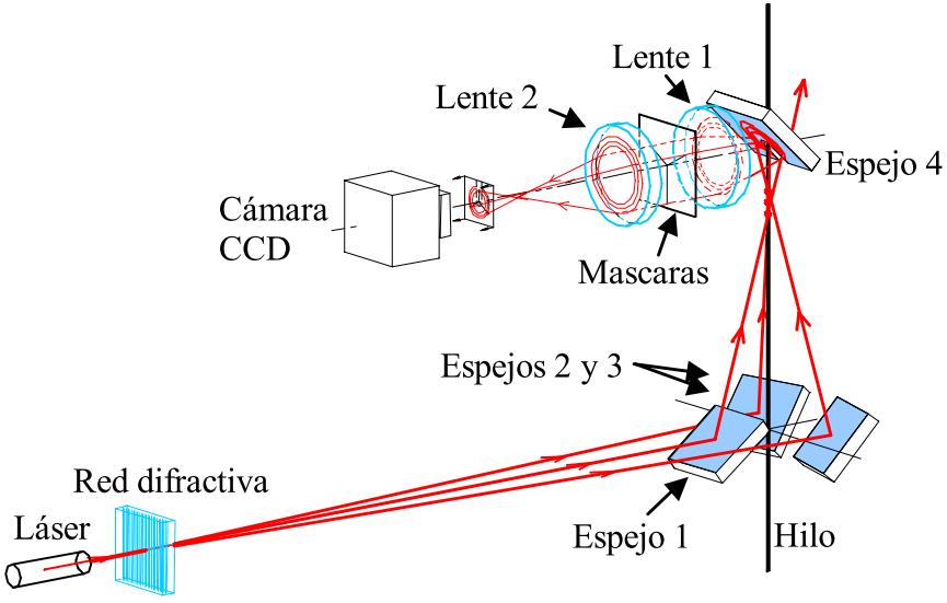	(b)	(c)
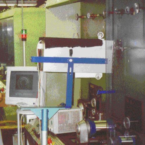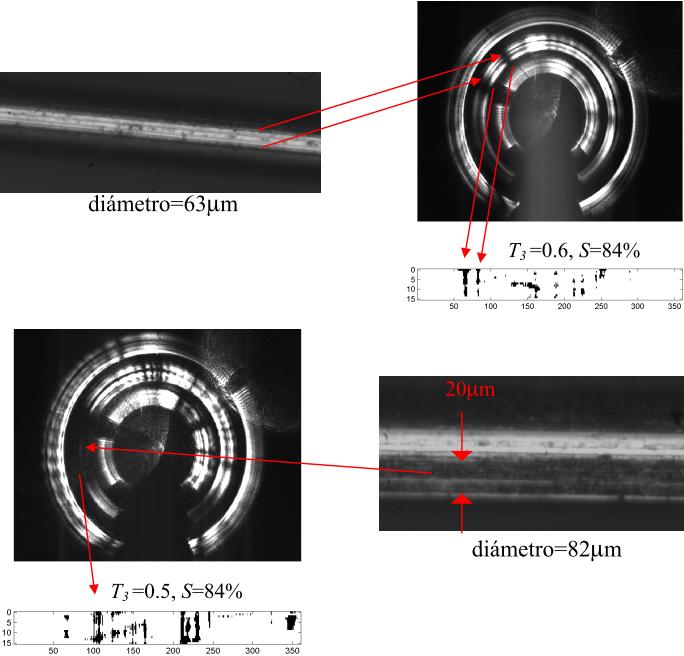
  Fig. 1. a) Optical device for 360º wire surface inspection (patent reference [1]). b) The surface defects are detected as fluctuations in the intensity profiles of the conical reflected beam.  c) Example of in-line implementation and image processing.

  
  
• Retroreflectivity measurements using a conventional color camera. We show a way to calibrate and measure with a conventional camera the retroreflectivity value of e.g. vertical traffic signs surfaces knowing either the area of the trafic sign surface or either the distance between the camera and the traffic sign surface. This method allows automatic retroreflectivity evaluation if the traffic sign could be automatically detected and recognized. See reference [5].
  

  (a)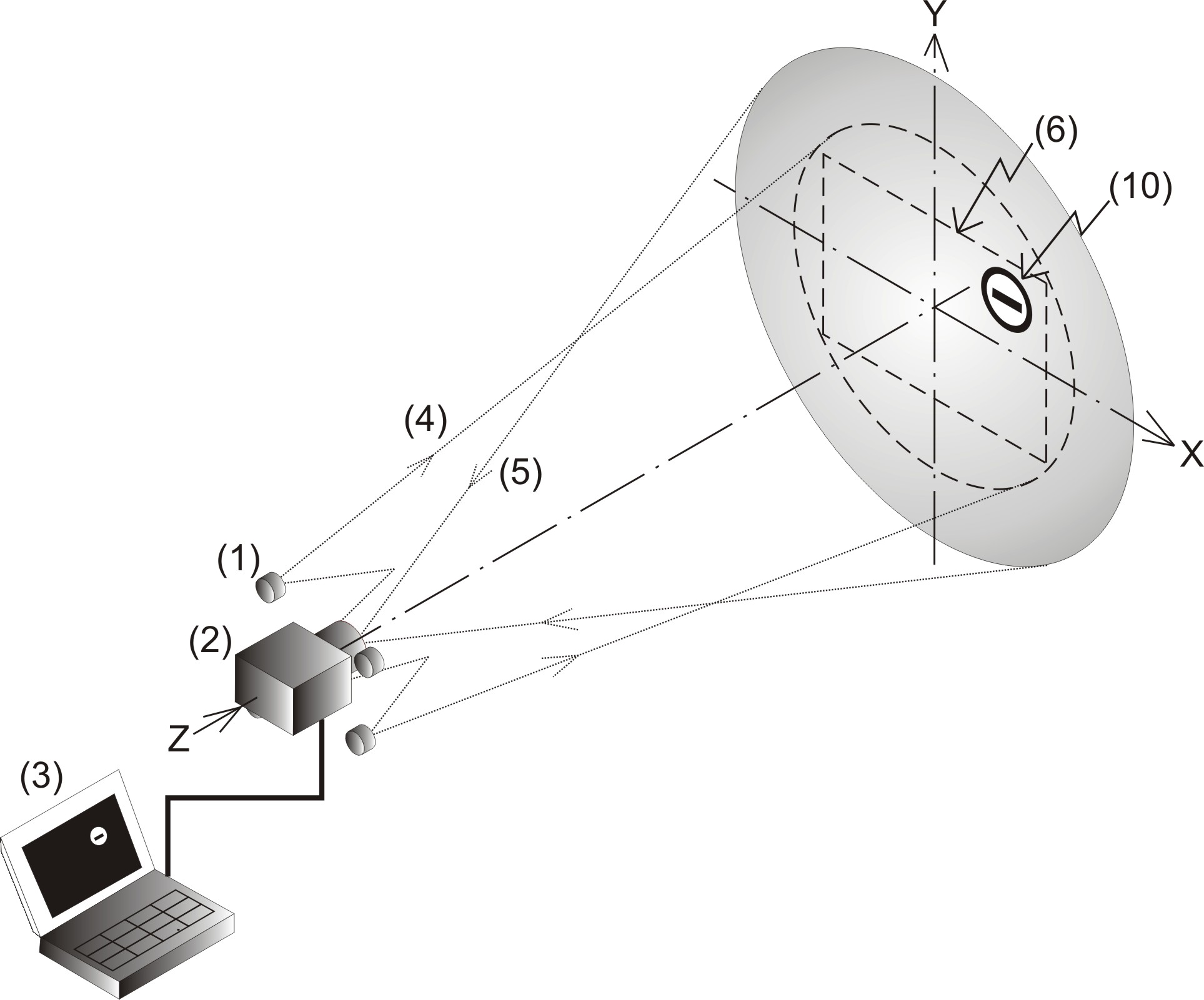	(b)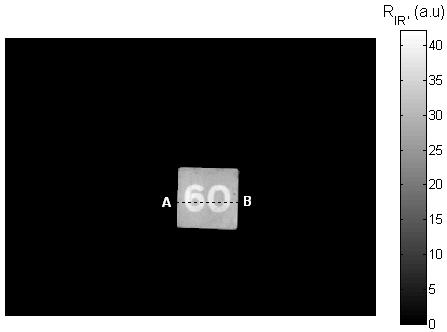	(c)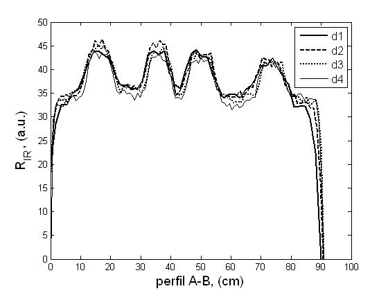
  Fig. 2. a) Scheme of the optical device for retroreflectivity measurements. b) Example of measured retroreflectivity of a traffic sign, and c) profile A-H at different distances to the device  (d1=20>d2>d3>d4=10m).

  
  
• Simultaneous in- and out-of-plane displacement measurements using one color camera and a color fringe projector. In Fig. 3(a), a self-calibrating device is presented for measuring in- and out-of-plane maps of displacements of a speckled specimen surface by using a combination of two well-known techniques such as fringe projection and two-dimensional digital image correlation. The device allows both: a precise perpendicular alignment with respect to a reference surface and a self-calibration (i.e. no calibration object is required) to obtain the required parameters for the calibration and correction of the observed displacements using two images of the reference surface with the camera displaced a known distance along the optical axis. The alignment and calibration procedure is computer aided by a guided user interface program that processes and displays the image to asses both the alignment and calibration. See reference [1], and patent 3.
  

  (a)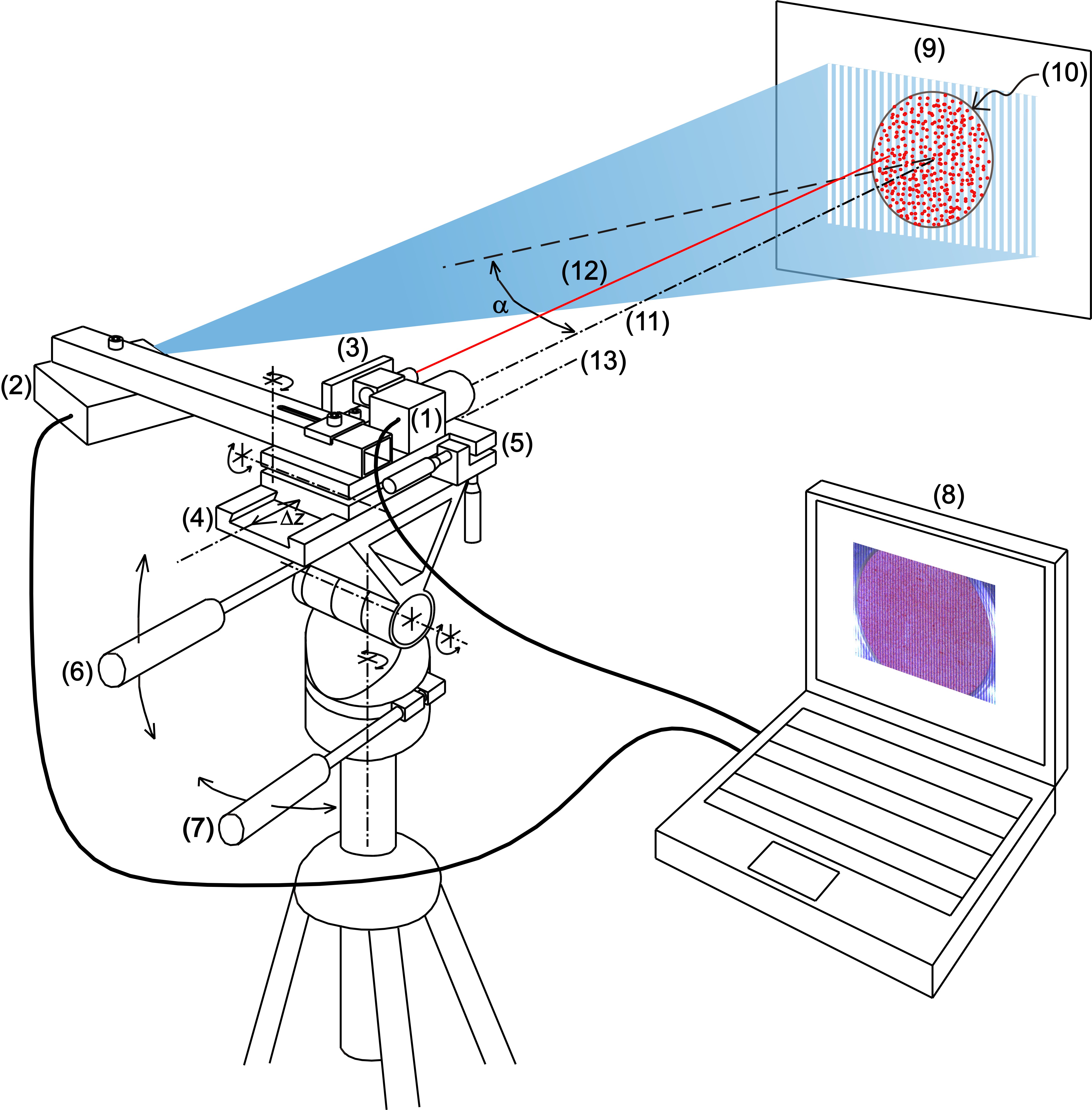	(b)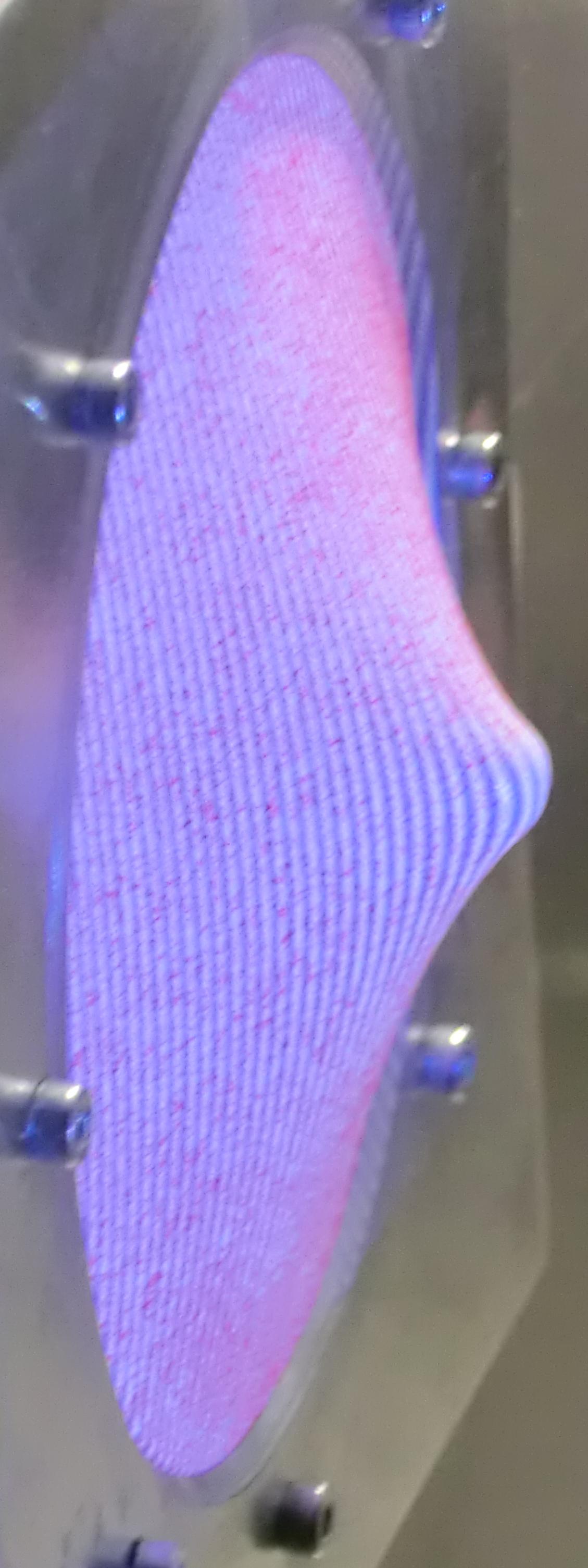	(c)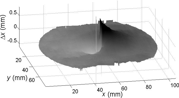 (d)	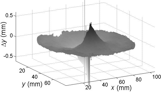(e)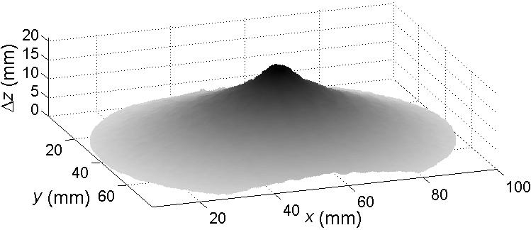
  Fig. 3. a) Scheme of the device for simultaneous measurements of in- and out-of-plane displacements. b) Example of a deformed elastic membrane and c) to e) the obtained displacements in each spatial direction.

  
  
• Image Processing for
• Digital Photoelasticity. We developed two new and quasy automatic methos for processing phase shifted digital images obtained from a monochromatic circular polariscope (for both reflection and transmission arrangements). Both methods deals with the ambiguity problem of the isoclinic angle in completely different ways. The first and faster one (called COPA)  performs a demodulation of the isoclinic phase map prior to obtain the  unambiguous isochromatic phase map, and the second and more robust but slower one (called RICO) regularizes directly the wrapped isochromatic phase map (result of a "José Castillejo" grant by the spanish "Ministerio de Ciencia y Educación" ). Both software can be downloaded here and the references explaining the algorithms  are [7] and [3] for COPA and RICO respectively.

  (a)	(b)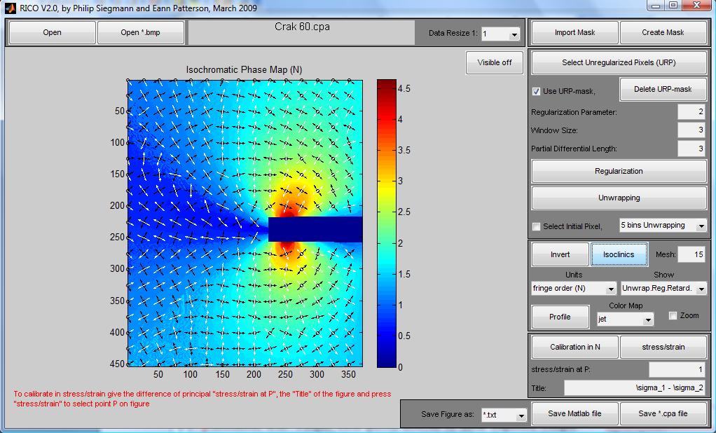
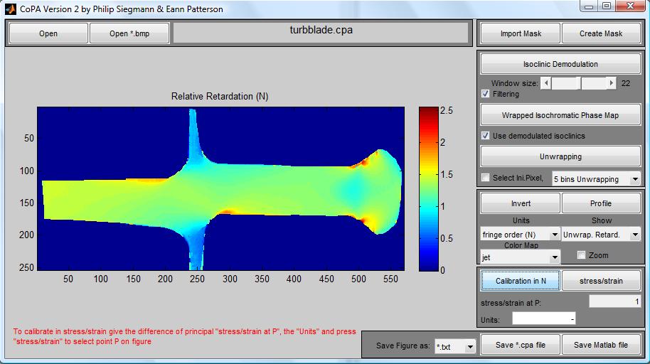
  Fig. 4. Grafic User Interface s of a) COPA and b) RICO (writen in MATLAB) showing examples of processed data: a)  section of a turbine blade and b) acrack propagation (CT test).

  
  
• Fringe Projection for 3D measurements.

  (a)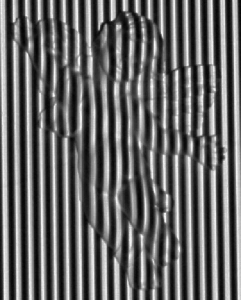	(b)
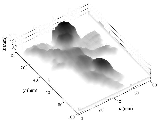  Fig. 5. a) Image of an angel with projected fringes. b) 3D reonstruction of the angel using 5 phase shifted Fringe Projection technique.

  
  
• Digital Image Correlation for in plane deformation measurements.
  

  (a)	(b)	(c)	(d)	(e)
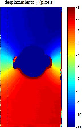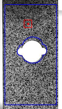
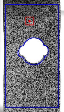
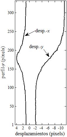
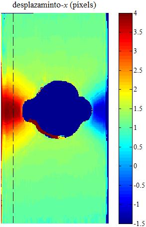
  Fig. 6. Example of 2D-DIC. a) Unloded sample. b) Verticaly streched sample. c) Profiles along the vertical lines shown on the x-displacement map (d) and y-displacement map (e).

• Signal Processing

• Nanoparticulate Air Pollution. This topic is a heritage of my dear oncle Hans Christoph Siegmann, who was dieply concerned and committed in providing us with a more healthy World. If I were able to get some finantial support I would be very happy to continue his work as I can, for example in the development of a multidimensional probabilistic source attribution model for a more precise detection and cuantification of air polluters.
  
• Field Measurements. Extremly high nanoparticulate air pollution measurements were obtained in Madrid in the years 1999 and 2000 which we published in [11]. Further measurements in Mexico City are shown in reference [9] as part of the "Air Pollution in the Mega-cities of the Developing World" project sponsored by the Alliance for Global Sustainability (AGS).
  
• Probabilistic Source Attribution (PSA), a method we have developed for detecting and quantifying (nanoparticulate) air polluters (see reference [6] and some comments in Alpha Galileo or SINC ).

  (a)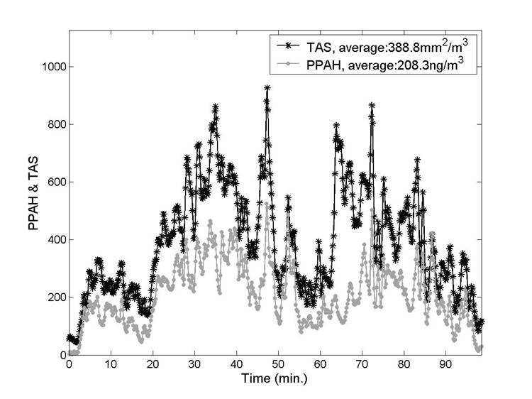	(b)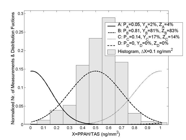
  Fig. 7. a) Example of a field measurement (TAS: Total Active Surface and PPAH: Particle-bound Polycyclic Aromatic Hydicarbons) along the roads of Madrid year 2006. b) By applying the PSA method to the measurements in (a), we obtain thant 81% of the measured data can be associated to source type B (fresh exhaust aerosol emmited from diesel vehicles).



• Kriging and Deconvolution Techniques: A way for approaching the "true signals" from sampled, convoluted and noisy data with uncertainity estimation. This is a topic I have just started to work at.

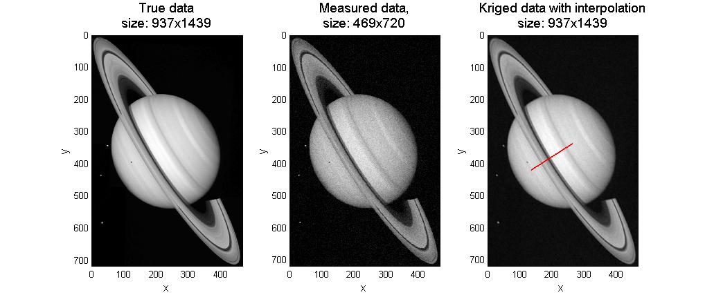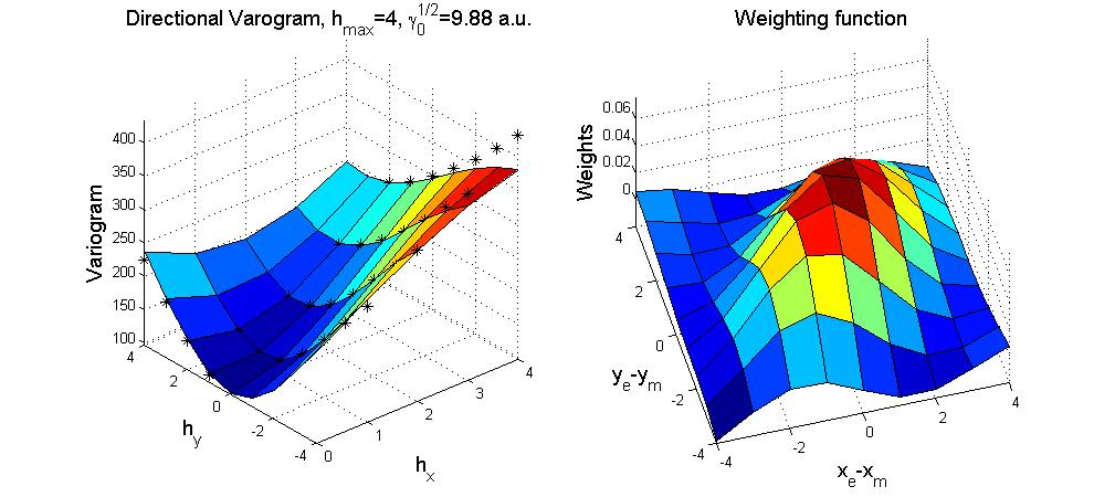
• Fig. 8. To estimate the true data from the measured data, we compute first the weigthing factors which are obtained from the directional variogram. The weighting factors are used to estimate the noise free values at any position. The measured data is sampled, noisy and also convoluted with the finite detector size (e.g. pixel size). After estimating a higher resoluted and noise free data a deconvolution is necesary if the true data is to be recovered.